Intro
We'll have a look at the minimization of dml functionals. The code can be checked out from this github repository. It is largely based on the multilayer perceptron code from the classic deep learning theano-dml tutorial, to which some convenient functionality to initialize, save and test models has been added. The basic testing functionality is explained in readme.md.
Getting started
After checking out the repository we will first create and save the parameters of the models generated by the modified multilayer perceptron. The key parameters are set at the top of the dml/mlp_test/mlp_modified.py script.
You can modify the defaults. If you are in a hurry or have time and/or a GPU for example, you can reduce/increase the number of epochs from the default 500 to 100 or to 1000 s in the Deeplearning tutorial. We will generate two series of saved models, one where the initial values are uniformly zero (randomInit=False above) and one where the initial values of the LogRegression layer are generated randomly (randomInit=True)
First
Looking into the dml/data/models you will see files containing the parameters of the models that have been saved, one every ten epochs, as per default. Then change to randomInit=True in mlp_modified.py and repeat.
Looking at the console output or at the logs you may realise that the randomly initialised sequence has at first lower error rates than the the one initialized with zeros. However the latter catches up after a while. In my test after 500 epochs the errors are respectively 178 and 174. Don't forget to set randomInit back to False if you intend to work with SdA later.
Plotting and interpreting the results
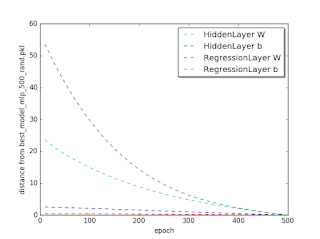
We will now see how the W and b of the HiddenLayer and of the RegressionLayer converge to their best model value, in this case the model corresponding to epoch 500. The distance that we consider is L2 norm. Using the methods in dml/mlp_test/est_compare_mlp_unit.py we get the plots.

We'll have a look at the minimization of dml functionals. The code can be checked out from this github repository. It is largely based on the multilayer perceptron code from the classic deep learning theano-dml tutorial, to which some convenient functionality to initialize, save and test models has been added. The basic testing functionality is explained in readme.md.
Getting started
After checking out the repository we will first create and save the parameters of the models generated by the modified multilayer perceptron. The key parameters are set at the top of the dml/mlp_test/mlp_modified.py script.
activation_f=T.tanh
n_epochs_g=500
randomInit = False
saveepochs = numpy.arange(0,n_epochs_g+1,10)
First
cd dml/mlp-test
python mlp_modified.py
python mlp_modified.py
Plotting and interpreting the results
We will now see how the W and b of the HiddenLayer and of the RegressionLayer converge to their best model value, in this case the model corresponding to epoch 500. The distance that we consider is L2 norm. Using the methods in dml/mlp_test/est_compare_mlp_unit.py we get the plots.

Distance from the 500-epoch parameters for the zero initialized model

Distance from the 500-epoch parameters for the random initialized model
We see that all four parameters converge uniformly to their best value. This may correspond to our naive expectations.
Now for the most interesting bit. Do the two model series approach the same optimum? Let's have a look at the next plot.
Now for the most interesting bit. Do the two model series approach the same optimum? Let's have a look at the next plot.

Distance from the zero and the random initialized model
It is apparent that the L2 distances between the parameters are not decreasing. They two series are converging to two different optima. It is actually well known that "most local minima are equivalent and yield similar performance on a testset", but seeing it may help.
No comments:
Post a Comment