Limit order book dynamics

The price changes triggered by a market order depend on the content the limit order  book.
A lob with constant depth yields a price change which is linear in the order size.

A lob with linearly increasing  depth yields a price change which is grows as the square root of the order size.

A lob with quadratically increasing  depth yields a price change which is grows as the cubic root of the order size.

And so on. . The code is here. Among the empirical values reported in the literature for the function's exponent I've found 0.5 and 0.76.

Spoofing, intention and AI

The 2010 Flash Crash wasn't a particularly glorious moment for the finance community. The search for culprits led to Navinder Singh Sarao , who ended up pleading guilty of spoofing (as well as of wire-fraud). As any high-frequency trader will tell you, spoofing, i.e. "placing bids with the intention of canceling them before they are executed", is a felony.

Now, let us consider the scenario sketched in my previous post and consider an AI-agent, let's say a dml-game-theoretic algorithm trained to maximize profits in a competitive environment . Will it spoof? Will it place "bids with the intention of canceling them before they are executed"?

Lawyers take note. AI-forensics is in its infancy (think of the Tesla car crash), but it will grow fast.

AI and the predictability paradox in finance

The no-arbitrage assumption is the bedrock of much of current financial markets modelling. At the same time time machine learning plays an increasing role in finance. Machine learning provides predictive capabilities which is highly relevant to financial trading. However, since every trade affects the market price of securities, effective predictions  destroy the assumption that financial markets are Markov processes. Let us consider a market where two or more players, each one striving to maximize  its profit, have predictive capabilities. Their strategies will impact and change the market. This will lead either to a winner take all situation or to an unpredictable crash-boom dynamics.
While the situation described is highly simplified, the underlying issue of free will (i.e. profit optimization) vs. predictability is real. The game-theoretic aspect will  be decisive. I am not aware of a theoretical framework dealing with this issue in quantitative terms (cf. [1]).

An interesting tidbit in this respect emerges from two quotes from this Bloomberg article about the Medaillon fund, reputedly the most successful of its kind: " ... we believe we have an excellent set of predictive signals, some of these are undoubtedly shared by a number of long/short hedge funds” and  "Too much money destroys returns. Renaissance currently caps Medallion’s assets between $9 billion and $10 billion" [2]. As trading algorithms predictions converge, managing their impact on the market becomes more difficult. As an aside for those who bother to read the whole article, Alexander Belopolsky is a member of the Theano development team.

[1] For a related philosophical discussion see e.g. S.Rummens, S.E.Cuypers "Determinism and the Paradox of Predictability" Erkenntnis, March 2010, Volume 72, Issue 2, pp 233–249. The instability scenario above relates to the "the typically oscillating nature of the paradoxical equation P = not-P" in [1] where traders "common causal history" are encoded in their trading strategies.

[2] Buying a security pushes up its price. Selling it pushes it down. The more one buys, the more one pays. The more one sells, the less one gets. The result is that, even admitting that the prediction about the the market is basically correct, the actual implementation of the strategy will distort the prices, the more so the bigger the volumes, as traders will heap up. At the same time the security price will return to its intrinsic value, penalizing any prediction based strategy. Determining the elasticity coefficients involved ins a highly relevant problem. See this paper by Gayduk and  Nadtochiy for a rigorous mathematical treatment of the issue.

MNIST and noMNIST - Theano and tensorflow

I warmly recommend Alec Radford's Theano-Tutorials to anyone interested in ML and Theano. His bare-bones approach yields remarkable clarity and effectiveness. I have adapted Alec's convolutional_net so that it works both with the MNIST dataset and on the noMNIST dataset used in the officoal tensorflow tutorial. The result is a remarkable 97.5% accuracy for the latter. To check it out you will have to build noMNIST.pickle and then place it in the data directory.  Besides,  comparing Theano and tensorflow may help understand each better.

MNIST naughties

After 500 epochs the multilayer perceptron fails on 33 of the MNIST training set images. Here are they. The y-label  is their array index, while the title contains the predicted value and the (obviously different) expected value according to MNIST.

The above image is was obtained running test_3(data_set='train') from mlp_test/test_mlp.py after creating and saving the model best_model_mlp_500_zero.pkl with mlp_modified-py. Some of the expected values are truly surprising. It is hard to see how 10994 (second row, first column) can be read as a 3. The trained network identifies it, imo correctly, as a 9. The same can be said of 43454 (5th row, 5th col) and of several other images. Some ones and sevens are hard to tell apart. . I've tried training the model on a training set where the naughty images above are replaced by duplicates from the rest of training set (see load_data in mlp_modified.py to see how it's done). However, this alone does not improve performance on the test set.

Wavelet denoising

I found this interesting post about wavelet thresholding on Banco Silva's blog. Unfortunately the code does not run under PyWavelets 0.4.0/Scipy 0.17.1 , but it inspired me to write a demo which does.

One pic says more than thousand words, so here it is:

As one can see, we add so much noise that the images practically disappear, but wavelet reconstruction (db8 in this case) is smart enough to recover the main features. The key point in the code is

threshold = noiseSigma * np.sqrt(2 * np.log2(noisy_img.size))
rec_coeffs = coeffs
rec_coeffs[1:] = (pywt.threshold(i, value=threshold, mode="soft") for i in rec_coeffs[1:])

Here soft thresholding  is used, where the wavelet coeffiicients whose absolute value is less than the threshold are assumed to be noise and hence set to zero, so as to denoise the signal. The other coefficients are shifted by sign*theshold so as to mantain the main patterns. Here a standard Donoho-Johnstone universal threshold is used. A look at the code may tell you more. 

Minima of dml functionals

Intro

We'll have  a look at the minimization of dml functionals. The code can be checked out from this github repository. It is largely based on the multilayer perceptron code from the classic deep learning theano-dml tutorial, to which some convenient functionality to initialize, save and test models has been added. The basic testing functionality is explained in readme.md.

Getting started

After checking out the repository we will first create and save the parameters of the models generated by the modified multilayer perceptron. The key parameters are set at the top of the dml/mlp_test/mlp_modified.py script.

activation_f=T.tanh
n_epochs_g=500
randomInit = False
saveepochs = numpy.arange(0,n_epochs_g+1,10)

You can modify the defaults. If you are in a hurry or have time and/or a GPU for example, you can reduce/increase the number of epochs from the default 500 to 100 or to 1000 s in the Deeplearning tutorial. We will generate two series of saved models, one where the initial values are uniformly zero (randomInit=False above) and  one where the initial values of the LogRegression layer are generated randomly (randomInit=True)
First

cd dml/mlp-test
python mlp_modified.py

Looking into the dml/data/models you will see files containing the parameters of the models that have been saved, one every ten epochs, as per default. Then change to randomInit=True in mlp_modified.py and repeat.

python mlp_modified.py

Looking at the console output or at the logs you may realise that the randomly initialised sequence has at first lower error rates than the the one initialized with zeros. However the latter catches up after a while. In my test after 500 epochs the errors are respectively 178 and 174. Don't forget to set randomInit back to False if you intend to work with SdA later.

Plotting and interpreting the results

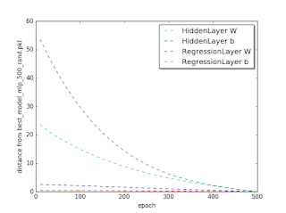
We will now see how the W and b of the HiddenLayer and of the RegressionLayer converge to their best model value, in this case the model corresponding to epoch 500. The distance that we consider is L2 norm. Using the methods in dml/mlp_test/est_compare_mlp_unit.py we get the plots.

Distance from the 500-epoch parameters for the zero initialized model

Distance from the 500-epoch parameters for the random initialized model

We see that all four parameters converge uniformly to their best value. This may correspond to our naive expectations.
Now for the most interesting bit. Do the two model series approach the same optimum? Let's have a look at the next plot.

Distance from the zero and the random initialized model

It is apparent that the L2 distances between the parameters are not decreasing. They two series are converging to two different optima. It is actually well known that "most local minima are equivalent and yield similar performance on a testset", but seeing it may help.